Difference between revisions of "4D Microscopy"
Montgomery (talk | contribs) |
Montgomery (talk | contribs) |
||
| Line 37: | Line 37: | ||
| − | <gallery widths= | + | <gallery widths=200px heights=200px> |
File:PFSM_2.png|Virtual probe plane formed by detection of the peak of the central interference fringe at each pixel in PFSM. | File:PFSM_2.png|Virtual probe plane formed by detection of the peak of the central interference fringe at each pixel in PFSM. | ||
</gallery> | </gallery> | ||
| Line 51: | Line 51: | ||
File:547ace0a460ecc0a6d7aee9f7f13bbf7.png | File:547ace0a460ecc0a6d7aee9f7f13bbf7.png | ||
</gallery> | </gallery> | ||
| − | Where C is a normalisation constant. | + | Where C is a normalisation constant. This formula provides a simple means of extracting the envelope of the interference fringes along the optical axis, the peak of which gives the position of the surface at a given pixel. The FSA algorithm is more robust than the PFSM algorithm, being less sensitive to variations in background intensity along the optical axis. |
| − | + | <gallery widths=200px heights=200px> | |
| − | + | File:FSA_1-bis.png|Calculation of the fringe visibility of the signal along the optical axis in FSA. | |
| − | <gallery widths= | + | File:FSA_2-bis.png|Detection of the peak of the envelope, giving the position of the surface at that point. |
| − | File:FSA_1-bis.png | ||
| − | |||
| − | File:FSA_2-bis.png | ||
</gallery> | </gallery> | ||
| − | |||
| − | |||
| − | |||
| − | |||
| − | |||
| − | |||
| + | While the FSA algorithm has a fixed sampling step of λ/8 between images, the axial resolution can be improved to about 10 nm by interpolation, using for example the least squares method. | ||
| − | ==== | + | ====Results and performance==== |
:Une mesure de grande taille (640 x 1024 pixels) "on-line" en utilisant l’algorithme de la PFSM est présentée ci-dessous, montrant le déplacement latéral d’une sonde microfluxgate (sonde magnétique intégrée). La mesure a été effectuée à une cadence de 1,9 images 3D par seconde sur une profondeur de 5 µm avec une résolution axiale de 40 nm. En diminuant la taille de l’image, la cadence de mesure peut être augmentée. <br/> | :Une mesure de grande taille (640 x 1024 pixels) "on-line" en utilisant l’algorithme de la PFSM est présentée ci-dessous, montrant le déplacement latéral d’une sonde microfluxgate (sonde magnétique intégrée). La mesure a été effectuée à une cadence de 1,9 images 3D par seconde sur une profondeur de 5 µm avec une résolution axiale de 40 nm. En diminuant la taille de l’image, la cadence de mesure peut être augmentée. <br/> | ||
Revision as of 15:37, 11 August 2023
4D Microscopy
- The aim of 4D microscopy is to measure and characterize moving or aperiodically changing microscopic structures (MEMS, nanotechnologies, engraving, chemical etching…) using interference microscopy. Our approach is to continuously scan the interference fringes over the whole of the depth of the surface to be measured, to capture the images with a high speed camera and to perform the image processing using highly parallel cabled logic to measure the height of the surface (see « Principle » page). (see « Principe » page).
The CAM 4D project
- The first 4D prototype system was financed by the ACO-CNRS project ("La microscopie optique 3D en temps réel à très haute résolution spatiale") and EU INTERREG III project, in which we succeeded in making measurements in real time at a rate of 6 3D images per second over a depth of several µm [A. Dubois et al., European Phys. J.: Appl. Phys., 2002]. The high speed camera developed in the laboratory allowed an acquisition rate of 250 images/s (512x512 pixels) and the processing was performed using an FPGA ("Field Programmable Gate Array") board.
- Thanks to the CAM4D project financed by Oséo, we were then able to develop a second prototype based on a high speed CMOS camera (500 i/s full field, 16000 i/s with reduced field) with improved real time performance, up to 25 3D images per second over a depth of several µm.
The measurement system
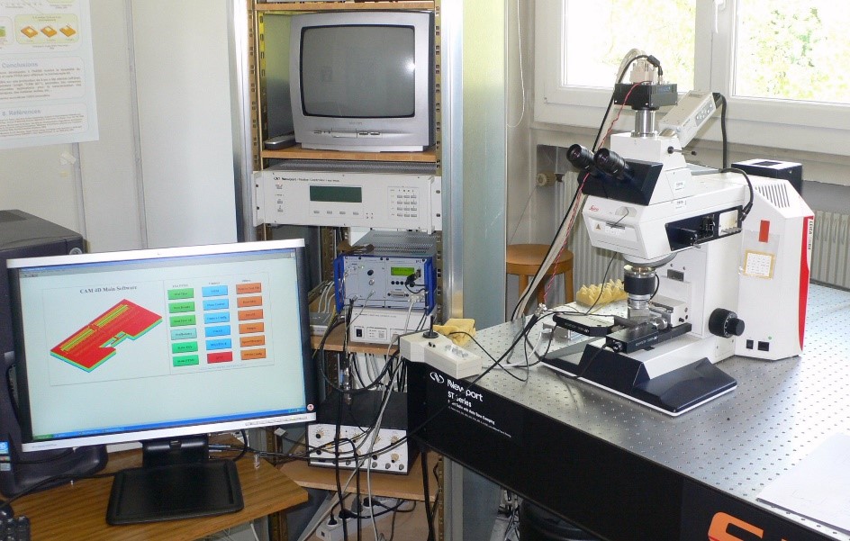
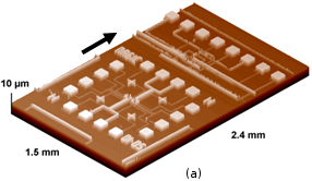
- The prototype consists of two parts. The first one is the Leica DMRX optical microscope equipped with interference objectives (Michelson or Mirau), a light source, a high speed camera, and a piezoelectric vertical translation stage with a range of 100 µm. The latter element is used to scan the fringes over the depth of the sample, the fringes appearing on the camera image of the sample surface. The second part consists of the acquisition board (equipped with a Virtex 2P FPGA Xilinx processor and SRAM or DDR memory) and the PC which controls the translation systems, the image acquisition and storage and the data processing. The whole system has to be carefully synchronised in order for it to function correctly.
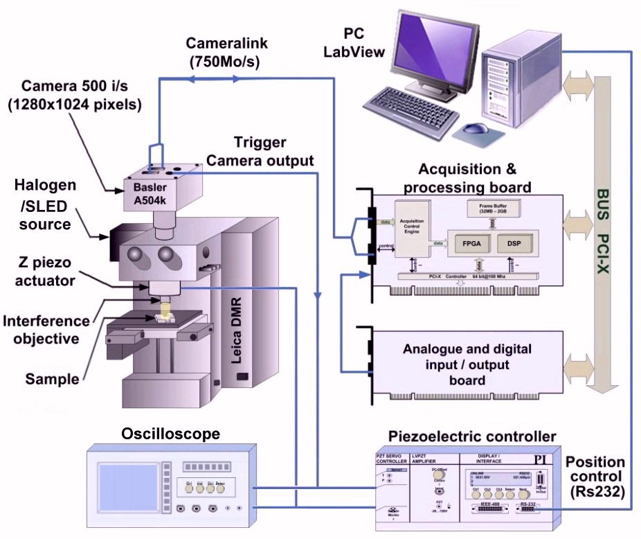
Layout of 4D microscopy system in the CAM4D project.
The 4D microscopy system.
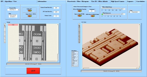
The visualisation software for viewing the results of the CAM 4D system.
- The microscope is placed on a vibration isolation table (SmartTable from NewPort) equipped with a dynamic compensation system to reduce residual vibrations. The scanned fringe images are sent via a « CameraLink » cable to the acquisition board to be processed by the FPGA, where the information about the height at each pixel is extracted. The results are then sent to the PC, where they are visulaised in 3d and analysed. The system has the advantage of being flexible in terms of the choice of the image size, the acquisition rate, the depth to be measured and the type of algorithm used.
The software for controlling the system, for visualising the results and analysing and storing them were developed in a LabView environment.
The algorithms
- The algorithms chosen were very compact, requiring only basic operators such as comparators, additions, multiplexers and multipliers that could be easily implemented in the FPGA. Two algorithms for extracting the surface height in real time were developed in VHDL (Very High speed integrated circuit hardware Description Language) and implemented in the FPGA: PFSM (Peak Fringe Scanning Microscopy) and FSA (Five-Sample-Adaptive non linear algorithm).
PFSM
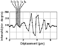
- The PFSM algorithm is very simple, consisting of detecting the peak intensity of the fringe signal, corresponding to the zero order fringe. This fringe peak is used as a virtual probe plane by detecting the highest intensity value at each pixel along the optical axis to measure the positon of the surface at each point and thus the 3D shape. The smaller the sampling step, the higher is the axial resolution but at the cost of more data to process.

Virtual probe plane formed by detection of the peak of the central interference fringe at each pixel in PFSM.
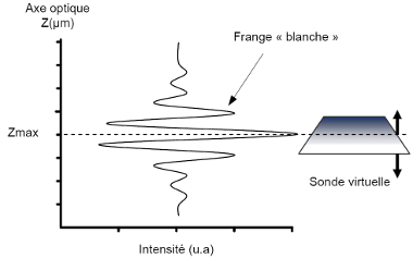
- The PFSM algorithm is well adapted to real time processing on the FPGA since it is fast enough to be applied during the image acquisition. It also has the advantage of being able to vary the axial resolution, typically from 10 nm to 100 nm. The disadvantage of the simplicity is the lack of robustness to variations in background intensity over the scan depth which should not present values higher than the fringe to be detected.
FSA
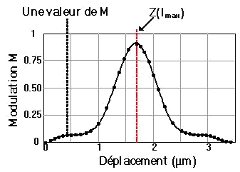
- The FSA (five Sample Adapative) algorithm consists of detecting the envelope of the fringes by measuring the fringe visibility at each point along the optical axis with a sliding window of 5 consecutive images with phase steps of 90° (λ/8) between images, corresponding to steps of about 76 nm at an average effective wavelength of λ = 610 nm. The following formula is used to calculate the fringe visibility or modulation:
Where C is a normalisation constant. This formula provides a simple means of extracting the envelope of the interference fringes along the optical axis, the peak of which gives the position of the surface at a given pixel. The FSA algorithm is more robust than the PFSM algorithm, being less sensitive to variations in background intensity along the optical axis.

Calculation of the fringe visibility of the signal along the optical axis in FSA.

Detection of the peak of the envelope, giving the position of the surface at that point.
While the FSA algorithm has a fixed sampling step of λ/8 between images, the axial resolution can be improved to about 10 nm by interpolation, using for example the least squares method.
Results and performance
- Une mesure de grande taille (640 x 1024 pixels) "on-line" en utilisant l’algorithme de la PFSM est présentée ci-dessous, montrant le déplacement latéral d’une sonde microfluxgate (sonde magnétique intégrée). La mesure a été effectuée à une cadence de 1,9 images 3D par seconde sur une profondeur de 5 µm avec une résolution axiale de 40 nm. En diminuant la taille de l’image, la cadence de mesure peut être augmentée.
- Fig. 6: Déplacement de la sonde ; (a) I0 : t = 0 s ; dx = 0 µm, (b) I8 : t = 8/1,9 = 4,21 s ; dx = 36 pixels = 84,6 µm
- Nous avons déplacé l’échantillon à l’aide d’une platine motorisée XY de précision. La vitesse de déplacement nominale de la platine est de 20 µm/s. Dans la figure 5, la sonde s’est déplacée de 84,6 µm (mesuré avec notre logiciel de profilométrie) sur un temps comprenant 8 images 3D, ce qui correspond à 4,21 secondes puisque la cadence de mesure 3D est de 1,9 images par seconde. On arrive alors à une vitesse de déplacement de la platine de 84,6/4,21 = 20,1 µm/s, ce qui correspond à la vitesse nominale.
- La mesure quantitative du relief de l’échantillon est une autre information fournie par les images d’altitude. La figure 6 montre le profil de la sonde magnétique intégrée. On observe que la profondeur mesurée est de 3,22 µm.

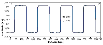
- Fig. 6: Mesure du profil de la sonde magnétique
- Des mesures en temps réel ont pu être réalisées au laboratoire et ont permis de valider le fonctionnement des algorithmes de la PFSM et de la FSA et les performances du système (figure 7). Les cadences de mesure d’images 3D sont données en fonction de la profondeur mesurée pour différentes tailles d’image. Ainsi, pour une image de 640 x 1024 pixels, il est possible d’atteindre une cadence 3D de mesure de quelques images par seconde. Avec une réduction de la taille d’image à 320 x 256 pixels, par exemple, la cadence 3D de mesure peut être augmentée à une vingtaine d’images par seconde. La résolution de la FSA doit être de 76 nm, mais le pas de la PFSM peut varier. Si le pas de la PFSM est augmenté, alors la cadence d’images 3D est elle aussi augmentée. En contrepartie, plus le pas de la PFSM est petit et meilleure sera sa résolution axiale.

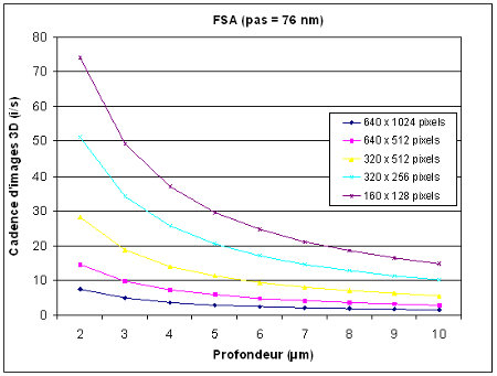
- Fig. 7: Les performances du système de mesure en temps réel
Les avantages du système CAM 4D
Le système de mesure 4D temps réel de l’InESS a l’avantage d’avoir une grande souplesse en termes de choix de taille d’images (les grandes tailles sont possibles), de cadence d’acquisition (caméra rapide pouvant monter à très haute cadence), de profondeur de mesure et de type d’algorithme employé (PFSM ou FSA). La microscopie par interférométrie 4D telle que développée à l’InESS comporte principalement trois avantages par rapport à la microscopie classique 3D. Le premier est qu’elle permet d’analyser un échantillon plus rapidement qu’en 3D classique. Le second, qui est le plus important, est qu’elle permet de visualiser et de quantifier des changements de surface en temps réel. Le troisième est que ceci est possible sur de grandes profondeurs d’analyse.
- Les points forts du système CAM 4D sont énumérés ci-dessous :
- Souplesse
- Choix de la taille de la surface à analyser (possibilité de grandes tailles) ;
- Choix de la cadence d’acquisition ;
- Choix de la profondeur de mesure ;
- Choix de l’algorithme à appliquer
- Algorithmes évolutifs : implémentés en logique câblée (FPGA) reprogrammable ;
- Logiciel de gestion modulaire du banc de mesure : développé sous LabView ;
- Logiciel de gestion modulaire du banc de mesure
- Banc constitué de composants standards (microscope, caméra rapide, carte de traitement, etc) ;
- Possibilité de déplacer soit l’objectif interférentiel ou soit l’échantillon ;
- Mesures 3D en temps réel enregistrables ;
- Mesure et caractérisation de structures microscopiques en mouvement périodique ou apériodique ;
- Cette technologie et principalement ces avantages ouvrent donc la voie vers de nouvelles applications.